Wave-based Non-Line-of-Sight Imaging in Julia
|
Keith Rutkowski ⋅
|
Introducing non-line-of-sight (NLOS) imaging
Imagine being able to take a three dimensional image of a room without having to enter it. That seems like a rather unbelievable accomplishment, but it is slowing becoming a reality with the technologies being developed in computational imaging, particularly non-line-of-sight imaging. Even though compact, commercialized forms of the technology are still a ways off in the future, it is already possible to build a "camera" to collect the data with today’s technology.
The process of capturing NLOS image data is fairly similar to taking regular image data, and while there are numerous variations of the approach, they all share the same components. First, there is an opening to the scene, like a doorway or window into a room, through which the camera can observe a surface within the scene, like a wall, floor, or ceiling.

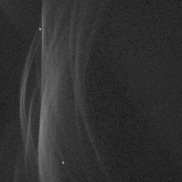
Then a "flash" is used to illuminate the scene. In the case of NLOS imaging, that flash is a high power laser. That light bounces around the scene, reflects off the observed surface, and eventually enters the camera. The vertical-temporal image below shows the laser "flash" bouncing around the scene and returning to the imaging surface as various wavefronts.
The camera has lenses and a shutter to collect light only during some particular period of time. Most cameras you have used capture light over \(1/60^{th}\), or perhaps even \(1/300^{th}\), of a second duration, but NLOS cameras need to capture light more precisely than that. They collect light over picosecond durations, that’s \(1/1000000000000^{th}\) of a second!
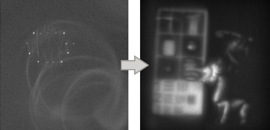
NLOS imagers need such small exposure times because they are actually recording the light patterns that form on a surface within the scene. When the laser illuminates the scene, its light travels throughout the scene and creates patterns of illumination on the observed surface. If you have ever observed patterns of light on the bottom of a swimming pool or sandy lake bottom, it is a similar effect.
You might be thinking that recording strange patterns of light doesn’t seem very useful, but that is precisely the kind of data being collected by a NLOS imager. While images of light wave patterns is nice and all, that doesn’t really live up to the hype of capturing images of hidden objects in a scene. Read on to see how 3D images can be formed from such apparently useless data.
3D scene reconstruction algorithms
There are many ways to form a 3D image from a sequence of light wave patterns, so we list some of the approaches below along with key highlights of each method:
-
Filtered Backprojection [Velten et al. 2012] [Gupta et al. 2012] [La Manna et al. 2018] [Arellano et al. 2017]
-
only gives approximation of shapes and reflectances
-
assumes only diffuse reflectance
-
ignores multi-bounce light paths
-
computationally costly, \(O(N^{5})\) algorithm
-
-
Light Cone Transform [O’Toole et al. 2018a]
-
assumes diffuse reflectance
-
requires confocal measurements (each image pixel needs to emit the laser from it)
-
lower computational cost, \(O(N^{3}\log(N))\) algorithm
-
-
Fast f-k Migration [Lindell et al. 2019]
-
capable of both diffuse and specular reflection
-
lower computational cost, \(O(N^{3}\log(N))\) algorithm
-
lower code complexity
-
Comparing the methods, you can see why we selected the fast f-k migration algorithm for implementation. It is accurate, requires less software development effort, and can run quickly on a desktop.
A Julia implementation of f-k migration
We implemented in Julia the fast f-k migration algorithm presented at SIGGRAPH 2019 in Wave-based non-line-of-sight imaging using fast f−k migration [Lindell et al. 2019] to reconstruct 3D images from the NLOS image data. The algorithm involves four rather simple steps:
-
Calibrate the collected data.
-
Transform the data.
-
Using Stolt interpolation, resample along the temporal frequency dimension.
-
Inverse transform the data to reconstruct the 3D scene.
We also need some NLOS imagery to try out our implementation of the algorithm, so we obtained datasets collected and published by the Stanford Computational Imaging Lab. It is the same data used in [Lindell et al. 2019] as well.
Calibration adjusts each pixel for the time it takes the light to travel from the observed surface to the camera. At the picosecond time scales captured in the NLOS image data, the travel time of light is non-negligible, so even if a light wave simultaneously illuminates the entire imaging surface, the camera would actually observe what appears to be a wave of light washing across the surface. Therefore, calibration is a very important step to processing the data.
The video on the right shows NLOS imagery and how the light wave patterns progress over time. The curved "black curtain" moving from right to left at the end of the video is a result of calibration and the different distances light had to travel for each pixel.
The three dimensions of the measured imagery, \(\tau(x,y,t)\), are the horizontal and vertical pixel counts of the imaging surface, \(X\) and \(Y\) respectively, and number of temporal samples, \(T\). To calibrate, each pixel’s vector of \(T\) samples must be shifted by its calibration time.
(X, Y, T) = size(tau)
for x in 1:X, y in 1:Y
  delay = floor(Int, calib[x, y] / 32)
  tau[x, y, :] .= circshift(tau[x, y, :], -delay)
end
Now the first time sample of each pixel corresponds to the exact same point in time at the imaging surface rather than at the camera. In seismic or acoustic applications of f-k migration, it is possible to acquire the image as phase and amplitude data, and in fact the algorithm assumes that data exists. However, in our application the wavelengths are too short to measure phase and amplitude effectively, so \(\tau(x,y,t)\) is an image of light intensity rather than amplitude and phase.
We must, therefore, convert to an amplitude image, \(\Psi(x,y,t)\), using the inverse of the relationship above as our first transform. Next, we pad the amplitude image with zeros, apply a Fourier transform, and shift the frequency data to be centered on the zero-frequency.
Psi = zeros(eltype(tau), map(s -> 2*s, size(tau)))
for t in 1:T
  Psi[1:X, 1:Y, t] .= sqrt.(tau[1:X, 1:Y, t])
end

PhiBar = fftshift(fft(Psi))
With our imaging data in the frequency domain, \(\bar{\Phi}(x,y,f)\), we are ready to apply Stolt interpolation. You can think of Stolt interpolation as curving the data in the way that wavefronts are curved as they reflect from a surface. Before continuing though, we wish to point out that Stolt interpolation has a significant drawback: it is based on the assumption that waves travel at the same velocity throughout the entire scene. This is a limitation to consider when modeling acoustic wave propagation where density can significantly affect velocity, but it is an acceptable assumption for our application of the technique to visible light propagation.
We implement the interpolation function, \(\Phi(x,y,f)\), in the following snippet of Julia code. Being careful to convert indices to a common unit for proper application of Stolt migration and avoid divide-by-0 situations are both key to getting the correct results. As you can see, we opted to create a couple of helper functions rather than stuff all the code into a large loop block.
function stoltLinearInterpZ(A, x, y, z)
  zLow  = floor(Int, z)
  zHigh = ceil(Int, z)
  low   = 1 <= zLow  <= size(A, 3) ? A[x, y, zLow] : 0
  high  = 1 <= zHigh <= size(A, 3) ? A[x, y, zHigh] : 0
  return low*(zHigh-z) + high*(z-zLow)
end

function stoltInterp(A, x, y, z; physX, physY, resT)
  i = 2*(x-1)/size(A, 1) - 1
  j = 2*(y-1)/size(A, 2) - 1
  k = 2*(z-1)/size(A, 3) - 1

  i *= (size(A, 1)/2*c*resT) / (4*(physX/2))
  j *= (size(A, 2)/2*c*resT) / (4*(physY/2))

  l = sqrt(i^2 + j^2 + k^2)
  f = (l + 1)*size(A, 3)/2 + 1
  S = max(c/2 * k/max(l, eps()), 0)
  return k > 0 ? S*stoltLinearInterpZ(A, x, y, f) : 0
end

Phi = zero(PhiBar)
for K_x in 1:size(Phi, 1), K_y in 1:size(Phi, 2), K_z in 1:size(Phi, 3)
  Phi[K_x, K_y, K_z] = stoltInterp(PhiBar, K_x, K_y, K_z, physX = 2, physY = 2, resT = 32e-12)
end
Finally, we bring the data back from the frequency domain with an inverse shift and inverse Fourier transform. The last detail is to crop the volume to remove the padding and apply the intensity-amplitude relationship to reconstruct the 3D image.
Psi = ifft(ifftshift(Phi))
tau = abs2.(Psi[1:X, 1:Y, 1:T])
It is rather impressive how few lines of code it takes to reconstruct a full 3D image from the data collected, isn’t it? So let’s take a look at the results of running the code against the "teaser" dataset to produce an image.
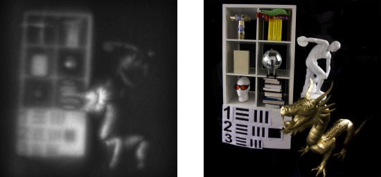
Honestly, the quality is probably on par with a 40 year old digital camera. On the other hand, it hopefully means that in about 40 years we will have GoPro’s with this capability strapped to our helmets showing us what’s around the corner before we even get there!
If you are interested in trying it out for yourself, grab the source code from GitHub along with some datasets from the Stanford Computational Imaging Lab. We hope you enjoyed the post, thanks for reading!
References
-
[Lindell et al. 2019] David B. Lindell, Gordon Wetzstein, and Matthew O’Toole. 2019. Wave-based non-line-of-sight imaging using fast f−k migration. ACM Trans. Graph. 38, 4, 116.
-
[O’Toole et al. 2018b] Matthew O’Toole, David B. Lindell, and Gordon Wetzstein. 2018b. Real-time non-line-of-sight imaging. ACM SIGGRAPH Emerging Technologies.
-
[O’Toole et al. 2018a] Matthew O’Toole, David B. Lindell, and Gordon Wetzstein. 2018a. Confocal non-line-of-sight imaging based on the light-cone transform. Nature 555, 7696 (2018), 338.
-
[Kirmani et al. 2009] Ahmed Kirmani, Tyler Hutchison, James Davis, and Ramesh Raskar. 2009. Looking around the corner using transient imaging. Proc. ICCV.
-
[Velten et al. 2012] Andreas Velten, Thomas Willwacher, Otkrist Gupta, Ashok Veeraraghavan, Moungi G. Bawendi, and Ramesh Raskar. 2012. Recovering three-dimensional shape around a corner using ultrafast time-of-flight imaging. Nature communications 3 (2012), 745.
-
[Gupta et al. 2012] Otkrist Gupta, Thomas Willwacher, Andreas Velten, Ashok Veeraraghavan, and Ramesh Raskar. 2012. Reconstruction of hidden 3D shapes using diffuse reflections. Optics Express 20, 17 (2012), 19096–19108.
-
[Arellano et al. 2017] Victor Arellano, Diego Gutierrez, and Adrian Jarabo. 2017. Fast back-projection for non-line of sight reconstruction. Optics Express 25, 10 (2017), 11574–11583.
-
[La Manna et al. 2018] Marco La Manna, Fiona Kine, Eric Breitbach, Jonathan Jackson, Talha Sultan, and Andreas Velten. 2018. Error backprojection algorithms for non-line-of-sight imaging. IEEE Trans. Pattern Anal. Mach. Intell. (2018).
 Keith Rutkowski is a seasoned visionary, inventor, and computer scientist with a passion to provide companies with innovative research and development, physics-based modeling and simulation, data analysis, and scientific or technical software/computing services.
He has over a decade of industry experience in scientific and technical computing, high-performance parallelized computing, and hard real-time computing.
Keith Rutkowski is a seasoned visionary, inventor, and computer scientist with a passion to provide companies with innovative research and development, physics-based modeling and simulation, data analysis, and scientific or technical software/computing services.
He has over a decade of industry experience in scientific and technical computing, high-performance parallelized computing, and hard real-time computing.